Re

https://www.youtube.com/watch?v=uzJXeluCKMs

1D

analysis of a system (calculations and the graphical approach): fixed points, stabilities
understand where exponential growth and decay come from
understand the logistic equation
linear stability analysis (perturbation close to a fixed point) – linearisation (Taylor)
existence and uniqueness
identify inertial and dissipative (damping) terms in a dynamical equation
know how to determine the potential (and the related stuff)

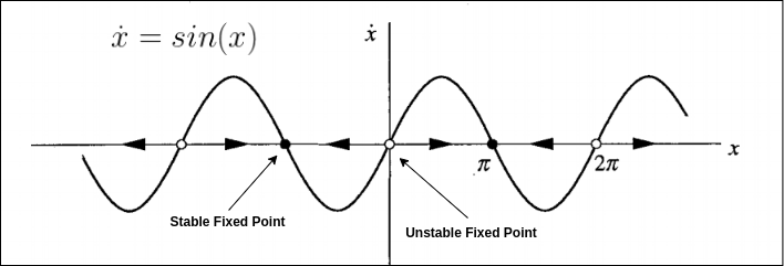
Vector fields

$\dot{x} > 0$ flow moves to the right
$\dot{x} < 0$ flow moves to the left

Stability

Two types of FPs:

Stable fixed points (attractors, sinks): flow converges towards them
Unstable fixed points (repellers, sources): flow goes away from them

Logisitc equation

$$ \dot{N} = rN \left( 1 - {N \over K} \right) $$

Linear stability analysis

Linearisation about $x^*$.
$f’(x^*) > 0$ grows exponentially → fixed point unstable
$f’(x^*) < 0$ decays exponentially → fixed point stable
$f’(x^*) = 0$ nonlinear analysis needed

Existence and uniqueness

definition
If $f(x)$ is smooth, solutions exist and are unique.

Potentials

If f(x) is well behaved (e.g. continuous), it is integrable, so one can introduce the potential V(x) of “the force” f(x) $$ f(x) = - { \mathrm{d} V \over \mathrm{d} x} \\ { \mathrm{d} V \over \mathrm{d} t} = { \mathrm{d} V \over \mathrm{d} x} { \mathrm{d} x \over \mathrm{d} x} = - \left( { \mathrm{d} V \over \mathrm{d} x} \right)^2 \leq 0 $$
Minimum of $V \to { \mathrm{d}^2 V \over \mathrm{d} x^2}$ > 0 \to f’(x) < 0 \tp$ stable fixed point
Maximum of $V \to { \mathrm{d}^2 V \over \mathrm{d} x^2}$ < 0 \to f’(x) > 0 \tp$ unstable fixed point

Bifurcations in 1D:

learn the normal forms and to identify different bifurcations that may occur
construction of a bifurcation diagram – and identification of a bifurcation based on it
splitting of a hard equation in two to ease the analysis
always be aware about linearisation and the accompanying analysis, e.g. approximation using the first two terms of the Taylor expansion (and be mindful about where the expansion is made – around FP and/or about bifurcation point)
Bifurcation: Qualitative change of the dynamics due to variation of a (control) parameter

Saddle-node bifurcation

NO fixed points → 1 Fixed point → 2 fixed points

Normal forms

$\dot{x} = r - x^2$
$\dot{x} = r + x^2$
taylor expansion about $x^*, r_c$ to get normal form

Transcritical bifurcation

normal form $\dot{x} = rx - x^2$
fixed points don’t disappear but switch stability

Pitchfork bifurcation

Supercritical pitchfork bifurcation

normal form: $\dot{x} = rx - x^3$
Left-right symmetry: The equation is invariant under the change of variables x → -x (left-right symmetry).
Supercritical: bifurcating FPs are stable.

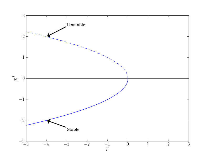
Subcritical pitchfork bifurcation

normal form: $\dot{x} = rx + x^3$
destabilizing term $+ x^3$
x ≠ 0 to infinity in a finite time when r > 0 (blow-up)

Flows on the circle

$$ \dot{\theta} = f(\theta) $$

$\theta$ = point on the circle
$\dot{\theta}$ = angular velocity at the point
can oscillate
particle can eventually return to starting position - periodicity

2D

Nullclines

fixed pointes in 1D
$f’(x^*) = 0$ and $g’(y^*) = 0$ independently
cross between nullclines = fixed point!!

Linear classification of FP

If the fixed point is not one of the borderline cases = centers, degenerate nodes, stars, non-isolated fixed points

Fixed points and linearization

Robust cases – linear analysis gives the FP correctly

Repellers (or sources): both eigenvalues have positive real part
Attractors (or sinks): both eigenvalues have negative real part
Saddles: one eigenvalue is positive, the other is negative

Marginal cases - linearisation fails, so the full system must be analysed

Centres: both eigenvalues are purely imaginary
Higher-order and non-isolated fixed points: at least one eigenvalue is zero

Marginal cases are those where at least one eigenvalue satisfies Re(λ) = 0.

Linearization

Jacobian $$ J = \begin{pmatrix} \frac{\partial f}{\partial x} & \frac{\partial f}{\partial y} & \ldots \\ \frac{\partial g}{\partial x} & \frac{\partial g}{\partial y} \\ \vdots & & \ddots \end{pmatrix} $$

$$ A = \begin{pmatrix} a & b \\ c & d \end{pmatrix} \\ \text{trace: }\tau = a + d = \lambda_1 + \lambda_2 \\ \Delta = \det A = ad - cb = \lambda_1 \lambda_2 $$

Eigenvalues and eigenvectors

$$ \lambda_{1,2} = \frac{\tau \pm \sqrt{\tau^2 - 4 \Delta}}{2} $$

$\lambda_i < 0$ = stable (= decays exponentially = arrow towards FP)
$\lambda_i > 0$ = unstable (= grows exponentially = arrow from FP)
$|\lambda_i| < |\lambda_j|$
- $\lambda_i$ = slow direction
- $\lambda_j$ = fast direction

Complex eigenvalues

if $\tau^2 - 4 \Delta < 0$ ⇒ complex solution
$\lambda_{1,2} = \alpha \pm i \omega$, $\qquad \alpha = { \tau \over 2 }, \omega = { \sqrt{4 \Delta - \tau^2} \over 2}$

Transition to polar coordinates

Used when the system results in borderline case when doing linear analysis.

Polar coordinates ⇒ Cartesian coordinates

$x = r \cos \theta$,
$y = r \sin \theta$

Cartesian coordinates ⇒ Polar coordinates

$r^2 = x^2 + y^2$
$r \dot{r} = x \dot{x} + y \dot{y}$
$\dot{\theta} = \frac{x \dot{y} - \dot{x} y}{r^2}$

Conservative systems

The energy is conserved.
Potential energy $V(x)$: $$ F(x) = - {\mathrm{d} V \over \mathrm{d} x} $$
trick to remember: multiply by $\dot{x}$ $$ m \ddot{x} = F(x) \\ F(x) = - {\mathrm{d} V \over \mathrm{d} x} \quad \to \quad m \ddot{x} + {\mathrm{d} V \over \mathrm{d} x} = 0 \\ m \dot{x} \ddot{x} + {\mathrm{d} V [x(t)] \over \mathrm{d} x} \dot{x} = 0 \\ \implies {\mathrm{d} \over \mathrm{d} x} \left[ \frac{1}{2} m \dot{x}^2 + V(x) \right] = 0 $$ Constant of motion $E = \frac{1}{2} m \dot{x}^2 + V(x)$
General definition
A conservative system cannot have any attracting fixed points.
In conservative systems trajectories are (typically) closed curves defined by contours of constant energy.

Reversible systems

For example, think of a pendulum.
time-reversal symmetry: their dynamics looks the same whether time runs forward or backward
$m \ddot{x} = F(x)$ is symmetric under time reversal $t \to -t \longrightarrow \ddot{x} \to \ddot{x}$ (velocity changes sign!)
any second-order system $$ \dot{x} = f(x,y) \\ \dot{y} = g(x,y) $$ such that $f$ is odd in $y$, $f(x, -y) = -f(x,y)$, and $g$ is even in $y$, $g(x, -y) = g(x,y)$ is reversible.
for a reversible system a linear center is alsoa nonlinear center.
Theorem (nonlinear centers for reversible systems): Suppose the origin x∗ = 0 is a linear center of a reversible system. Then, sufficiently close to the origin, all orbits are closed.
General reversibility definition

Nondimensionalization

https://en.wikipedia.org/wiki/Nondimensionalization#math_1

$$ { \mathrm{d}^2 \theta \over \mathrm{d} t^2 } + { g \over L } \sin \theta = 0 $$

Nondimensionalization: $\omega = \sqrt{g \over L}, \tau = \omega t$

$$ \boxed{ \begin{align*} { g \over L } &= \omega^2 \\ t = { \tau \over \omega }, \mathrm{d} t = \frac{1}{\omega} \mathrm{d} \tau \to { \mathrm{d} \tau \over \mathrm{d} t} &= \omega \\ { \mathrm{d} \over \mathrm{d} t } = { \mathrm{d} \tau \over \mathrm{d} t } { \mathrm{d} \over \mathrm{d} \tau } &= \omega { \mathrm{d} \over \mathrm{d} \tau } \\ \to \left( { \mathrm{d} \over \mathrm{d} t } \right)^n = \left( \omega { \mathrm{d} \over \mathrm{d} \tau } \right)^n &= \omega^n { \mathrm{d}^n \over \mathrm{d} \tau^n } \end{align*} } $$

$$ \begin{align*} &{ \mathrm{d}^2 \theta (t) \over \mathrm{d} t^2 } &&+ { g \over L } \sin \theta(t) &&= 0 \\ \to & \omega^2 { \mathrm{d}^2 \theta \left( {\tau \over \omega} \right) \over \mathrm{d} \tau^2 } &&+ \omega^2 \sin \theta \left( {\tau \over \omega} \right) &&= 0 & /\cdot \frac{1}{\omega^2} \\ \to & { \mathrm{d}^2 \theta \left( t( \tau ) \right) \over \mathrm{d} \tau^2 } &&+ \sin \theta \left( t( \tau ) \right) &&= 0 \\ \to & { \mathrm{d}^2 \Theta( \tau ) \over \mathrm{d} \tau^2 } &&+ \sin \Theta ( \tau ) &&= 0 \end{align*} $$

Index theory

Index theory definitions
The vector field makes one complete rotation counterclockwise, so $I_C = +1$.
The vector field makes one complete rotation clockwise: $I_C = −1$.
Trick: The index is the net number of counterclockwise revolutions made by the numbered vectors in (b).

Limit cycles

A limit cycle is an isolated closed trajectory: neighbouring trajectories either spiral away from it or towards it.
If neighbouring trajectories tend towards the limit cycle, the latter is called stable or attracting, otherwise unstable, in exceptional cases it may be half-stable.
Limit cycles are typical features of nonlinear systems: in linear systems there are periodic orbits, but they are not isolated!

By Hannes Vogel - Own work, CC BY-SA 4.0, Link

learn everything that you need to recognize and analyse limit cycles
understand what relaxation oscillations are
this applies to other parts (that is, other Lectures) as well: make sure you know what different parts in a second-order differential equation do: dissipation, inertia, …
the different tools/theorems for analysis - what having a gradient system means/implies, Liapunov function, Dulac, Poincaré-Bendixson, etc. – are important
you should understand the reason for relaxation oscillations, but you are not expected to remember hard calculations. Qualitative understanding at the level of the diagram on page 36 suffices; if you are to do some analysis, you will be given equations or clear hints what you should be explaining

Gradient systems

$\bold{\dot{x}} = - \nabla V$, $V(x)$ = single-valued scalar function
No inertial ($\propto \ddot{x}$) components in gradient systems.
Sufficient condition for a system to be gradient: $$ \boxed{ \begin{align*} \dot{x} = f(x, y), \\ \dot{y} = g(x, y), \\ { \partial f(x, y) \over \partial y } = { \partial g(x,y) \over \partial x } \end{align*} } $$
There can’t be closed orbits in gradient systems: Let us assume there is $\implies \nabla V = 0$ $$ \nabla V = \int_0^T {\mathrm{d} V \over \mathrm{d} t } \mathrm{d} t = \int_0^T \left( \nabla V \cdot \bold{\dot{x}} \right) \mathrm{d} t = - \int_0^T \bold{\dot{x}} \cdot \bold{\dot{x}} \mathrm{d} t = - \int_0^T || \bold{\dot{x}} ||^2 < 0 $$ Contradiction.

Dissipation

A dynamical equation can be divided in energy and its dissipation.
$\ddot{x} + (\dot{x})^3 + x = 0$
Energy function: $E(x, \dot{x}) = \frac{1}{2} (x^2 + \dot{x}^2)$
related to energy = $\ddot{x}$ and $x$
related to dissipation = $\dot{x}$

Lyapunov functions

Energy-like functions that decrease along trajectories.
$\bold{\dot{x}} = f(\bold{x})$, $\bold{x}^*$ is a fixed point.
A Lyapunov function s a continuously differentiable function $V(\bold{x})$ such that:
1. $V(\bold{x}) > 0$, $\bold{x} \neq \bold{x}^∗$ and $V(\bold{x}^∗) = 0$ ($V$ is positive definite).
2. $\dot{V} < 0$, for all $\bold{x} \neq \bold{x}^∗$. (All trajectories flow towards $\bold{x}^∗$.)

If there is such a function, $\bold{x}^∗$ is globally asymptotically stable: for all initial conditions $\bold{x(t)} \to \bold{x}^∗$, when $t \to \infty$. Consequently, the system has no closed orbits.

Solutions cannot get stuck anywhere else, because if they did, V would stop changing, which would contradict 2).

sometimes sum of squares work: $V(x,y) = x^2 + ay^2$, $\dot{V} = 2x\dot{x} + 2 a y \dot{y}$

Poincaré-Bendixson theorem

defintion
Standard trick: Construct a trapping region, i.e. a region on whose boundary the vector field points inwards…

Relaxation oscillations

These oscillations are characterised by repetitious slow build up and sudden discharge.
$\ddot{x} + \mu (x^2 - 1) \dot{x} + x = 0, \mu \gg 1$
Use lienard transformation instead of standard trick $$ \ddot{x} + \mu (x^2 - 1) \dot{x} = {\mathrm{d} \over \mathrm{d} t} [\dot{x} + \mu (\frac{1}{3} x^3 - x)] \\ F(x) = \frac{1}{3} x^3 - x \\ w = \dot{x} + \mu F(x) \\ \implies \dot{x} = w - \mu F(x) \\ \dot{w} = -x \\ \text{let use } y = { w \over \mu } \\ \implies \\ \boxed{ \begin{align*} \dot{x} &= \mu [y - F(x)] \\ \dot{y} &= - \frac{1}{\mu} x \end{align*} } $$

Bifurcations in 2D

prototype normal forms in 2D
understand characteristics of different bifurcations in 2D including the Hopf bifurcation
Poincaré maps

Saddle-node bifurcation

prototypical example: (same as 1D but add stable manifold in $y$-axis - exponential decay) $$ \dot{x} = \mu - x^2 \\ \dot{y} = - y $$

Transcritical and pitchfork bifurcations

transcritical $\dot{x} = \mu x - x^2, \dot{y} = -y$
supercritical pitchfork $\dot{x} = \mu x - x^3, \dot{y} = -y$
subcritical pitchfork $\dot{x} = \mu x + x^3, \dot{y} = -y$

Hopf bifurcations

two complex-conjugate eigenvalues
only for space n >= 2

Supercritical Hopf bifurcation

a stable spiral ➔ an unstable spiral
Trick to remember : rewrite to Cartesian coordinates + Jacobian and eigenvalues from Jacobian $$ \dot{r} = \mu r - r^3 \\ \dot{\theta} = \omega + br^2 $$

Subcritical Hopf bifurcation

$$ \dot{r} = \mu r + r^3 - r^5 \\ \dot{\theta} = \omega + b r^2 $$

Identifying Hopf bifurcations

Supercritical, if a small attracting limit cycle appears immediately after FP goes unstable, and its amplitude shrinks back to zero as the parameter is reversed (no hysteresis).
Subcritical in most other cases. If hysteresis, then for sure.
Degenerate: For example, changing the damping μ from positive to negative in the damped pendulum $\ddot{x} + \mu \dot{x} + \sin x = 0$ turns FP at the origin from a stable to an unstable spiral. However, there are no limit cycles on either side of the bifurcation, but a continuous band of closed orbits surrounding (0,0). This is not a true Hopf bifurcation. Hopf typically happens when a nonconservative system becomes conservative at the bifurcation point: FP becomes a nonlinear centre, not a weak spiral.

Poincaré Maps

The Poincaré map converts difficult problems about closed orbits into much easier problems about fixed points of a mapping. (Although finding P may be impossible.)
definition $$ \phi’ = y \\ y’ = I - \sin \phi - \alpha y $$

When $I > 1$ there are no more FPs available. Claim: For $I > 1$, all trajectories are attracted to a unique, stable limit cycle. The first step to prove this is to show that a periodic solution exists. For this we need a Poincaré map.

How to do it

To show that $y^∗$ exists, we need to know what the graph roughly looks like. For a trajectory that starts at $y = y_1 , \phi = 0: P(y_1) > y_1$. For a trajectory that starts at $y = y_2 , \phi = 0: P(y_2) < y_2$.

Chaos in 3D

Learn the Lorenz system well. There will probably be one or more essay questions on this. Qualitative understanding of different regimes is expected (when changing the relevant parameter) – The Butterfly and the diagram on page 60.

Lorenz map
chaos (what it is – “definition”)
attractors – strange and regular
Lyapunov exponent must be remembered, you would need it to explain some aspect of chaos

Lorenz equations

$$ \dot{x} = \sigma (y - x) \\ \dot{y} = rx - y - xz \\ \dot{z} = xy - bz \\ \sigma, r, b > 0 $$

Prandtl number $\sigma$ is the ratio of the viscous to thermal diffusion,
Rayleigh umber $r$ is the ration of the driving to dissipation,
$b$ has no name

in a certain range of parameters σ, r, and b there could be no stable fixed points and no stable limit cycles
yet, all trajectories remain confined to a bounded region
moreover, all trajectories are eventually attracted to a set of zero volume

Basic properties

two non-linearities $xz$ and $xy$
Symmetry: $(x,y) \to (-x, -y)$

Volume contraction

The Lorenz system is dissipative: volumes in phase space contract under the flow.

$$ V(t + \mathrm{d} t) = V(t) + \int_S (\bold{f} \cdot \bold{n} \mathrm{d} t) \mathrm{d} A \\ \implies { V(t + \mathrm{d} t) - V(t) \over \mathrm{d} t } = \int_S (\bold{f} \cdot \bold{n}) \mathrm{d} A \\ \text{Divergence theorem} \to \dot{V} = \int_V \nabla \cdot \bold{f} \mathrm{d} V \\ \nabla \cdot \bold{f} = { \partial \over \partial x }[\sigma(y - x)] + { \partial \over \partial y }[rx - y - xz] + { \partial \over \partial z }[xy - bz] = - \sigma - 1 - b < 0 \\ \dot{V} = - ( \sigma + 1 + b ) V \\ \to V(t) = V(0) e^{ - ( \sigma + 1 + b ) } $$

Volumes in phase space shrink exponentially fast.
The Lorenz system cannot have repellers (unstable nodes or unstable closed orbits)! – repellers are sources of volume
Consequence: fixed points must be sinks or saddles, and closed orbits (if there are any) must be stable or saddle-like.

Fixed points

origin for all values of parameters
$r > 1$: a symmetric pair of fixed points left or right-turning convection rolls $C^+$ and $C^-$

Strange attractor

“Strange”: These attractors are often fractals.
has a fractal structure, that is if it has non-integer Hausdorff dimension

Chaotic strange attractor

A chaotic strange attractor is an attractor that exhibits sensitive dependence on initial conditions.
bounded set of zero volume -> chaos on a strange attractor
Lorenz’ butterfly
The number of circuits made on either side is unpredictable
Motion on the attractor exhibits sensitive dependence on initial conditions: two trajectories starting very close to each other will rapidly diverge from each other.
- Neighbouring trajectories separate exponentially fast!

Lyapunov exponent

$\lambda$ is Lyapunov exponent
- There are actually n different exponents, one for each “dynamically relevant” dimension; $\lambda$ is the largest of them.
- When $\lambda$ is positive, there is a time horizon beyond which prediction breaks down.
Let $||\delta_0||$ be the error of the initial state. The discrepancy between the estimate and the true state will grow exponentially, $||\delta|| \sim e^{\lambda t}$

Lorenz map

“some single feature of a given circuit should predict the same feature of the following circuit.”
“The single feature”: zn , the nth local maximum of z(t).

Lorenz’s idea: z n should predict zn+1. Numerical integration: zn+1 vs. zn appear to fall on a single curve.
The function $z_{n+1} = f(z_n)$ is called the Lorenz map.

One-dimensional maps

fixed points and cobwebs
Logistic map - characteristics
period-doubling bifurcation
chaos and periodic windows
orbit diagram (understanding it is important)
intermittency
Liapunov exponent
universality – what it is in the logistic map

Dynamical system, time is discrete, as opposed to previous stuff $$ x_{n+1} = \cos x_n $$
Sequence $x_0, x_1, x_2, \dots$ is the orbit starting from $x_0$
As tools for analyzing differential equations, As models of natural phenomena, As simple examples of chaos - Successful predictions of routes to chaos by using maps.

Fixed Points and Cobwebs

fixed point: $x_{n+1} = f(x_n) = f(x^) = x^$
stability of $x^*$
- $\lambda = f’(x^∗)$ is the eigenvalue or multiplier
- if $|\lambda| = |f’(x^)| < 1 \to x^$ is linearly stable.
  - For $\lambda = 0$ fp is superstable - extremely fast convergence
- if $|\lambda| = |f’(x^)| > 1 \to x^$ is linearly unstable.
- if $|\lambda| = |f’(x^*)| = 1$ marginal case needs higher-order term $O(\eta^2_n)$ to determine local stability
Cobweb particularly useful when linear analysis fails

Logistic map

$$ x_{n+1} = r x_n (1 - x_n), \quad x_n \geq 0, r \geq 0 $$

$x_n$ is a dimensionless measure of the population in the $n$th generation

Flip bifurcation

$f’(x^*) = -1$
has single stable fixed point and then
one unstable fixed point and one stable orbit of period two
example: $f(x) = \mu - x - x^2$

Period-Doubling

the population oscillates between n values - period-$n$ cycle

chaos and periodic windows

For many values of r the sequence {$x_n$} never settles down to a fixed point or a periodic orbit: a discrete-time version of chaos.
The periodic windows are interspersed between chaotic clouds of dots.
The blow-up (lower diagram) reveals self-similarity.

orbit diagram (understanding it is important)

Intermittency

Cobweb: The system takes a long time to pass through the channels between the diagonal and the curve; here $f^3(x) \sim x \to$ 3-cycle.

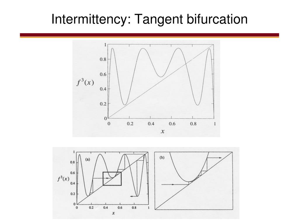
Tangent bifurcation

$f^3 (x)$ must have become tangent to the diagonal: the stable and unstable 3-cycles coalesce and annihilate in a tangent bifurcation.
tangent bifurcation = saddle-node bifurcation; (as r increases 3-cycle appears out of blue sky and splits into a stable and unstable 3-cycle)

Liapunov exponent

$$ \lambda = \lim_{n \to \infty} \left[ \frac{1}{n} \sum_{i=0}^{n-1} \ln \left| f’(x_i) \right| \right] $$

Universality

$\Delta_n = r_n − r_{n−1}$ = distance between consecutive bifurcation values.
$d_n$ is the smallest distance from the maximum of $f$, $x_m$ , to the nearest point in a $2^n$-cycle

Fractals and strange attractors

the Cantor set and topologically Cantor sets
fractal properties presented by the example sets: Cantor, von Koch curve
different ways to determine the dimension of a fractal object (set): similarity dimension, box dimension, correlation dimension
self-similarity
understanding on strange attractors and chaotic dynamics through properties of maps (e.g., baker’s and Hénon)

Fractal properties of cantor set

$C$ has structure at arbitrarily small scales.
$C$ is self-similar. $C$ “contains” smaller copis of itself at all scales.
The dimension of $C$ is not an integer. $dim C = \frac{\ln 2}{\ln 3} \approx 0.63$.

$C$ has a measure zero.
- $C = S_\infty$ is covered y each of the sets $S_n$
- The total length of $C$ is less than the total length of $S_n$.
- $L_0 = 1, L_1 = \frac{2}{3}, L_2 = \left( \frac{2}{3} \right)^2, \dots, L_n = \left( \frac{2}{3} \right)^n$
- The length of $C: L_\infty = lim_{n \to \infty} L_n = 0$
$C$ in uncountable.

Similarity Dimension.

$m$ is the number of copies
$r$ is the scale factor
dimension $d = { \ln m \over \ln r }$.
Definition: Suppose that a self-similar set is composed of $m$ copies of itself scaled down by a factor of $r$. Then the similarity dimension d is the exponent defined by $m = r^d$.

Box Dimension

generalise the notion of dimension to deal with fractals that are not self-similar.
“Measurement”: cover the set with boxes of size $\varepsilon$.
Let $S$ be a subset of $D$-dimensional Euclidian space, and let $N(\varepsilon)$ be the minimum number of $D$-dimensional cubes of side $\varepsilon$ needed to cover $S$.
$N(\varepsilon) \propto \frac{1}{\varepsilon^d}$
Definition of box dimension: $d = \lim_{\varepsilon \to 0} { \ln N(\varepsilon) \over \ln (1 / \varepsilon)}$, if the limit exists.

Pointwise and Correlation Dimension

Fix a point $\bold{x}$ on the attractor $A$
Let $N_x(\varepsilon)$ denote the number of points on $A$ inside a ball of radius $\varepsilon$ about $\bold{x}$
pointwise dimension $d$ at $\bold{x}$ in $N_\bold{x}(\varepsilon) \propto \varepsilon^d$
correlation dimension $d$ $C(\varepsilon) \propto \varepsilon^d$ to average $N_\bold{x}(\varepsilon)$ over many $\bold{x}$ to obtain an overall dimension of $A$.

The baker’s map

$0 \leq x \leq 1, 0 \leq y \leq 1$ $$ (x_{n+1}, y_{n+1}) = \begin{cases} (2x_n, ay_n) & 0 \leq x_n \leq \frac{1}{2} \\ (2x_n - 1, ay_n + \frac{1}{2}) & \frac{1}{2} \leq x_n \leq 1 \end{cases} $$ where $a$ is a parameter in the range $0 \leq a \leq \frac{1}{2}$

Hénon map

$$ x_{n+1} = y_n + 1 - a x_n^2 \\ y_{n+1} = b x_n $$ where $a$ and $b$ are adjustable parameters.

$$ T’:\\ x’ = x, \\ y’ = 1 + y - ax^2 \\ $$ $$ T’‘: \\ x’’ = bx’ \\ y’’ = y’ \\ $$ $$ T’‘’: \\ x’‘’ = y’’ \\ y’‘’ = x’’ $$ The composite transformation $T = T’‘’(T’‘(T’))$ yields the Hénon mapping.

Properties

invertible, trajectories are unique
dissipative - contracts areas at the same rate everywhere in phase psace (Jacobian)
the strange attractor is enclosed in the trapping region.

Cheat sheet setup

nullclines ($\dot{x} = 0$, $\dot{y} = 0$)
Fixed points = cross between nullclines
Classification of fixed points (stability, types, …)
- Jacobian = linear classification
Eigenvalues and eigenvectors
Reversible system, Conservative system, Potential function

By-heart

Definitions

Existence and uniqueness definition

Consider the initial value problem: $$ \dot{x} = f(x), \quad x(0) = x_0 $$ Suppose that $f(x)$ and $f’(x)$ are continuous on an open interval $R$ of the $x$-axis and that $x_0$ is a point in $R$. Then the initial value problem has a solution $x(t)$ on some time interval $(-τ, τ)$ about $t = 0$, and the solution is unique.

For the layman: If f(x) is smooth, solutions exist and are unique.

Manifolds definition

If a trajectory starts on the y-axis, the system’s state converges to x*: the y-axis is the stable manifold of the saddle point (i.e. initial conditions bringing the system to x*)

Stable manifold: the set where one ends up when starting at – in fact, infinitesimately close to $-x^*$ and running the dynamics backward in time ($t \to -\infty$) ; here the y-axis Trajectories starting off the y-axis converge asymptotically ($t \to \infty$) to the $x$-axis that is the unstable manifold

Unstable manifold: the set of initial conditions leading to $x^*$ when dynamics runs backward in time ($t \to -\infty$) ; here the $x$-axis

Manifold: A topological space, which is homeomorphic to Euclidian space $\mathbb{R}^m$ locally. (homeomorpism: there is a continuos function $f$ between spaces, and $f^{-1}$ exists)

Stability definition

$x^*$ is an attracting fixed point when all trajectories starting near $x^*$ approach it asymptotically: if all trajectories are attracted, the point is called globally attracting
$x^*$ is Lyapunov stable if all trajectories that start sufficiently close to $x^*$ remain close to it at any time
$x^*$ is neutrally stable if it is Lyapunov stable but not attracting: nearby trajectories are neither attracted nor repelled from the point (common in mechanical systems without friction: e.g. simple harmonic oscillator)
$x^*$ is stable (or asymptotically stable) if it is both Lyapunov stable and attracting
$x^*$ is unstable if it is neither Lyapunov stable nor attracting

Existence, uniqueness and topological consequences

Existence and Uniqueness Theorem: Consider the initial $$ \bold{\dot{x} = f(x)}, \qquad \bold{x}(t_0) = \bold{x_0} $$ Let $\bold{f}$ and all its partial derivatives ${ \partial f_i \over \partial x_j }, i,j = 1, \cdots, n$ be continuous for $\bold{x}$ in some open connected set $D \subset \mathrm{R}^n$. Then for $x_0 \in D$ the initial value problem has a solution $\bold{x}(t)$ on some time interval $(-\tau, \tau)$ about $t = 0$, and the solution is unique.

Corollary: different trajectories never intersect! If two trajectories did intersect there would be two solutions starting from the same point (the crossing point).

Consequence in two dimensions: any trajectory starting from inside a closed orbit will be trapped inside it forever! What will happen in the limit t → ∞ ? The trajectory will either converge to a fixed point or to a closed (periodic) orbit! (The last part: Poincaré-Bendixson theorem.)

Fixed points and linearization definition

If Re(λ) ≠ 0 for both eigenvalues, the fixed point is called hyperbolic: in this case its type is predicted by linearisation. The condition Re(λ) ≠ 0 is the exact analog of f’(x*) ≠ 0 in one dimension for the stability of the FP to be accurately predictable by linearisation. Re(λ) ≠ 0, of course, applies also in higher-order systems. Hartman-Grobman Theorem: The local phase portrait near a hyperbolic fixed point is topologically equivalent to the phase portrait of the linearisation. (In other words, there is a homeomorphism that maps one to the other.) Fixed points and linearization Homeomorpism: Let X1 and X2 be topological spaces. A map f : X 1 → X2 is a homeomorphism if it is continuous and has an inverse f -1 : X2 → X1 , which is also continuous. If there exists a homeomorpism between X1 and X2, X1 is said to be homeomorphic to X2 and vice versa. Examples: a) An open disc D2 = {(x, y) ∈homeomorphic to R2 . R2 | x 2 + y 2 < 1} is b) A coffee cup is homeomorphic to a doughnut. → Fixed points and linearization Intuitively, two phase portraits are topologically equivalent if one is a distorted (bending, warping, but not tearing) version of the other. Hence, closed orbits stay closed, trajectories connecting saddle points must not be broken, etc. A phase portrait is structurally stable if its topology cannot be changed by an arbitrarily small perturbation of the vector field. Hence, the phase portrait of a saddle point is structurally stable, that of a center is not, since a small perturbation converts the center into a spiral.

Conservative systems definition

Systems with a conserved quantity are called conservative. General definition: Given a system $\bold{\dot{x}} = f(x)$, a conserved quantity is a real-valued continuous function $E(\bold{x})$ that is constant on trajectories (${ \mathrm{d} E \over \mathrm{d} t } = 0$), but nonconstant on every open set (to exclude e.g. $E(x) \equiv 0$).

Reversibility definition

More general definition of reversibility: If there exists a mapping $R(\bold{x})$ of the phase space to itself that satisfies $R^2(\bold{x}) = \bold{x}$, then the system $\bold{\dot{x}} = f(\bold{x})$ is invariant under the change of variables $t \to −t$, $\bold{x} → R(\bold{x})$. (Reflection about the $x$-axis has the property $R^2(\bold{x}) = \bold{x}$.)

Index theory definition

Suppose a smooth vector field $\bold{\dot{x}} = f(\bold{\dot{x}})$ on the phase plane and consider a simple (= non-self-intersecting) closed curve $C$, which does not pass through fixed points of the system. Then at each point of $C$ the vector field makes a well-defined angle $\phi = \arctan( {\dot{y} \over \dot{x}})$ with the positive $x$-axis.

As $\bold{x}$ moves counterclockwise around $C$, the angle $\phi$ changes continuously (the vector field is smooth) → when $\bold{x}$ comes back to the starting position $\phi$ has varied by a multiple of $2 \pi$. $[\phi]_C$ = the net change in $\phi$ over one circuit The index of the closed curve C: $$ I_C = \frac{1}{2 \pi} [\phi]_C $$

Dulac’s criterion definition

Let x ሶ = f(x) be a continuously differentiable vector field on some simply connected subset R of the plane. If there exists a continuously differentiable, real-valued function g x such that ∇ ∙ g x ሶ has one sign throughout R, there are no closed orbits lying entirely in R. Proof: Let us assume that there is a closed orbit C lying entirely in R. A is the area within C. Green’s theorem Non-zero Zero, since Contradiction → no closed orbits.

Poincaré-Bendixson Theorem definition

A criterion to establish that closed orbits exist. Theorem: Suppose that:

R is a closed, bounded subset of the plane;
x ሶ = f(x) is a continuously differentiable vector field on an open set containing R;
R does not contain any fixed points;
There exists a trajectory C that is confined in R, i.e. it starts in R and stays in R for all future time . Then either C is a closed orbit or it spirals towards a closed orbit as t → ∞. ➔ Chaos cannot occur in the phase plane.

Poincaré Maps definition

General definition of a Poincaré map in an $n$-dimensional system $\bold{\dot{x}} = f(\bold{x})$. Let $S$ be an $n − 1$ dimensional surface of section that is transverse to the flow. The Poincaré map is a mapping from $S$ to itself, obtained by following trajectories from one intersection with $S$ to the next. The $k$th intersection $\bold{x}_k \in S$.

The Poincaré map: $$ \bold{x}_{k+1} = P(\bold{x}_k) $$

Chaos definition

There is no universally accepted definition of the term chaos, but a general agreement on the following three ingredients.

Chaos: aperiodic long-term behavior in a deterministic system that exhibits sensitive dependence on initial conditions

Aperiodic long-term behavior: trajectories do not settle down to fixed points, periodic orbits, quasiperiodic orbits as $t \to \infty$.
Deterministic: the system has no random or noisy inputs or parameters → the irregular behavior arises from nonlinearity.
Sensitive dependence on initial conditions: nearby trajectories separate exponentially fast → positive Lyapunov exponent.

Attractor definition

Definition: an attractor is a closed set $A$ with the following properties:

$A$ is an invariant set: any trajectory $\bold{x}(t)$ that starts in $A$ stays in $A$ for all time.
$A$ attracts an open set of initial conditions: there is an open set $U$ containing $A$ such that if $\bold{x}(0) \in U$, then the distance from $\bold{x}(t)$ to $A$ tends to zero as $t \to \infty$. So, $A$ attracts all trajectories that start sufficiently close to it. The largest such $U$ is called the basin of attraction of $A$.
$A$ is minimal: there is no proper subset of $A$ that satisfies conditions 1 and 2.